Wednesday, February 27, 2019
Response of First Order System – (Sinusoidal response)
 EXPERIMENT
Response of First Order System – (Sinusoidal
response)
1. EXCLUSIVE SUMMARY
The objective of this experiment is to
study the response of first order subjected to sinusoidal response. To achieve
this objective, the apparatus shown in the figure 2 was used. The maximum
temperature reached in the thermobath and thermowell are 50 ◦C and 42 ◦C
respectively. The minimum temperature reached in the thermobath and thermowell
are 32 ◦C and 36 ◦C respectively. The period of oscillation is 60 sec. Initial
amplitude and output amplitude of first order sinusoidal response is 9 ◦C and 3
◦C respectively. The amplitude of the system is 0.333. The frequency of
oscillation (ω) is 0.105 radian/sec. Time constant from amplitude ratio is
27.03 sec. the phase lag is 60 ◦C. time constant from phase lag is 3.05 sec.
2. INTRODUCTION
SINUSOIDAL INPUT- This function is represented mathematically by the
equations

Where
A is the amplitude and is the radian
frequency [1]. The radian frequency is related to the frequency f in cycles per
unit time by ω = 2πf. Figure 1 shows the graphical representation of this
function. The transform is


3. OBJECTIVE
To study the response of a first order system subjected to a
sinusoidal response.
4. Experimental Setup
 |
| First order sinusoidal set-up |
The apparatus consist
two thermometer. First thermometer is for thermowell and second is for
thermobath. Water is flowing continuously. Water level indicator is attached to
the vessel contacting heating coil.
5. Procedure
1. Start the clean water supply
by opening the inlet valve of heating bath and maintain constant water flow
through the heating bath. Keeping constant level in “Water head” indication
tube can ensure this.
2. Insert the thermometer and
thermo well in heating bath.
3. Ensue that cyclic timer is
set to @30 seconds on time and @30 seconds off time. Switch on Mains to heat
the water in heating bath.
4. After some time observe
sinusoidal response of the heating bath temperature on thermometer. The amplitude (temperature range) can be
changed by adjusting water flow rate and period can be changed by adjusting on
time, off time of the cyclic timer. (Period = On time + off time)
5. At steady state note
amplitude ratio and phase lag (Refer observations)
6. Results and Discussions
 |
Above figure shown the first order
sinusoidal response. Temperature of the bath and thermowell represent on the
y-axis and time on the x-axis. The maximum temperature reached in the
thermobath and thermowell are 50 ◦C
and 42 ◦C respectively. The
minimum temperature reached in the thermobath and thermowell are 32 ◦C and 36 ◦C respectively. The period of oscillation is 60
sec. Initial amplitude and output amplitude of first order sinusoidal response
is 9 ◦C and 3 ◦C respectively. The amplitude of
the system is 0.333. The frequency of oscillation (ω) is 0.105 radian/sec. Time
constant from amplitude ratio is 27.03 sec. the phase lag is 60 ◦C. time constant from phase lag
is 3.05 sec.
7. CONCLUSIONS
The maximum
temperature reached in the thermobath and thermowell are 50 ◦C
and 42 ◦C respectively. The minimum temperature reached in
the thermobath and thermowell are 32 ◦C and 36 ◦C
respectively. The period of oscillation is 60 sec. Initial amplitude and output
amplitude of first order sinusoidal response is 9 ◦C
and 3 ◦C respectively. The amplitude of the system is
0.333. The frequency of oscillation (ω) is 0.105 radian/sec. Time constant from
amplitude ratio is 27.03 sec. the phase lag is 60 ◦C.
time constant from phase lag is 3.05 sec.
8. REFERENCE
1. Coughanowr
D., LeBlanc S., ‘Process Systems Analysis and Control’, Mc-Graw Hill Science Engineering
Math, 2nd Edition, 2008, P-87-92.
1. Coughanowr
D., LeBlanc S., ‘Process Systems Analysis and Control’, Mc-Graw Hill Science
Engineering Math, 2nd Edition, 2008, P-92-97
RESPONSE OF 1ST ORDER SYSTEMS IN INTERACTING TANKS

EXPERIMENT
RESPONSE
OF 1ST ORDER SYSTEMS IN INTERACTING TANKS
EXECUTIVE SUMMARY
The objective of this
experiment is to study the dynamic response of first order in interacting
tanks. To achieve the objective, the system was given a step change and an
impulse change at 40 and 50 LPH. Initially the system was subjected to step
function which was performed by two ways, i.e. giving a step-up from 40-50 LPH
and a step-down from 50-40 LPH. Followed
by impulse input at 40 and 50 LPH by adding 500 ml of water. , the height of
tank 2 suddenly increases and then decreases to achieve steady state. For
impulse change higher the flow rates more fluctuation and more time to achieve
steady state. The time constant for impulse change at different flow rate were
same so there was no effect on changing flow rate. For higher order, transfer
lag required is more and the system requires more time to achieve the ultimate
value. The resistance of the tank 2 is in the range of (r2) = 0.266
and time constant is in the range of (τ2) = 0.001772 sec.
1. OBJECTIVE:
To study the response of
two non- interacting tank system subjected to step and impulse change
2. THEORY:
The variation in h2 in tank
2 does not affect the transient response in tank1. This type of system is
called non interacting system.
Applying mass balance on
tank 1 and tank 2:

3. EXPERIMENTAL SETUP
 |
| Setup of interacting tank |
The setup consists of two
transparent body tanks with graduated scales connected in interacting mode by a
resistance pipe. While performing the interacting tanks experiment, the pipe
connecting tank 1 and tank 2 is kept completely closed. A rotameter with
flowrates in LPH is used for the supply. The outlet of the rotameter is used to
fill up the tank. A pump is present which recycles the water.
4. PROCEDURE:
1)
Start up the set up.
2)
A flexible pipe is provided at the rotameter outlet. Insert
the pipe in to the cover of the top Tank 1. Keep the outlet valves (R1 &
R2) of both Tank 1 & Tank 2 slightly closed. Ensure that the valve (R3)
between Tank 2 and Tank 3 is fully closed.
3)
Switch on the pump and adjust the flow at 70 LPH. Allow the
level of both the tanks (Tank 1 & tank 2) to reach at steady state and
record the initial flow and steady state levels of both tanks.
4)
Apply the step change with increasing the rotameter flow by @
10 LPH.
5)
Record the level of Tank 2 at the interval of 3 sec, until
the level reaches at steady state.
6)
Record final flow and steady state level of Tank1
7)
Repeat the experiment by throttling outlet valve (R1) to
change resistance.
Impulse change:
1)
Set the flowrate of tank at 50 LPH and allow it to achieve
steady state.
2)
Add 500 mL of water in tank 1 suddenly and start the
timer.
3)
Observe the change in height of tank 2 with respect to time
(sec) and note it down after every 3 sec until steady state is achieved and
stop the timer 4) Repeat the above steps for 60 LPH.
5)
Empty the tanks.
6)
Switch off the pump.
5. RESULTS AND DISCUSSION:
 |
| level of tank vs time for impulse change at 40 LPM |
The above figure shown the
level of tank vs time for impulse change at 40 LPM (~litre per minute). Level
of tank is representing on the y-axis and time for impulse change represented
on the x-axis.
It is dome in shape. The
height of tank 2 suddenly increases and then decreases to achieve steady state
value. Maximum height attained is 15 mm when flowrate is 40 LPH.
 |
| level of tank vs time for impulse change at 50 LPM |
It is dome in shape. The
height of tank 2 suddenly increases and then decreases to achieve steady state
value. Maximum height attained is 14 mm when flowrate is 50 LPH. The time to
achieve steady state at higher flow rate is higher for impulse change.
 |
| level of tank vs time for step change 40 LPM |
 |
| level of tank vs time for step change |
The above figure 4 and 5
epresents the response curve for interacting system subjected to step change.
Figure 3 is for step-up from 40 LPH where the height of the tank 2 increases
linearly with increase in time. Figure 4 is for step-down from 50 LPH where the
height of the tank decreases linearly with increase in time.
As the time increases the
level in the tank increase and achieve steady state. The resistance of the tank
2 is in the range of (r2) = 0.266 and time constant is in the range
of (τ2) = 0.001772 sec.
6. CONCLUSION
The aim is to study the
response of first order interacting system subjected to impulse and step
change. The height of tank 2 increases and decrease with time respectively. But
for impulse, the height of tank 2 suddenly increases and then decreases to
achieve steady state. For impulse change higher the flow rates more fluctuation
and more time to achieve steady state. The time constant for impulse change at
different flow rate were same so there was no effect on changing flow rate. For
higher order, transfer lag required is more and the system requires more time
to achieve the ultimate value. The resistance of the tank 2 is in the range of
(r2) = 0.266 and time constant is in the range of (τ2) =
0.001772 sec.
7. REFERENCES:
Coughanowr D., LeBlanc S., ‘Process Systems Analysis and Control’, Mc-Graw Hill Science Engineering
Math, 2nd Edition, 1991, Pg 228-238.
Inherent characteristics of control valve

Inherent
characteristics of control valve
1. EXCLUSIVE SUMMARY
The objective of this experiment is to
study the inherent
characteristics of control valve. To achieve this objective, the apparatus
shown in the figure 1 was used. An equal percentage valve overcompensates for
line loss and produces an effective characteristic that is not linear, but is
bowed in the opposite direction to that of the effective characteristic of the
linear valve. One can show that as the line loss increases, the linear valve will
depart more from the ideal linear relation and the equal percentage valve will
move more closely toward the linear relation. Pressure drop of water in equal%,
quick opening and linear valve are in the range of 101.2 -147.6, 33.6-147.6 and
83.6- 147.6 mm respectively.
2. INTRODUCTION
The control valve is
essentially a variable resistance to the flow of a fluid, in which the
resistance and therefore the flow, can be changed by a signal from a process
controller.
The function of a control
valve is to vary the flow of fluid through the valve by means of a change of
pressure to the valve top. The relation between the flow through the valve and
the valve stem position (or lift) is called the valve characteristic.
In general, the flow
through a control valve for a specific fluid at a given temperature can be
expressed as:

where,
q = volumetric flow rate
L = valve stem position (or
lift)
po = upstream pressure
pt = downstream pressure
The inherent valve
characteristic is determined for fixed values of pa and p 1.

where,
qmax is the maximum flow
when the valve stem is at its maximum lift L (valve is full-open)
x is the fraction of maximum
lift
m is the fraction of maximum
flow.
m = q/q(max) =f(L/L(max))
The types of valve
characteristics can be defined in terms of the sensitivity of the valve, which
is simply the fractional change in flow to the fractional change in stem
position for fixed upstream and downstream pressures.
sensitivity = dm/dx
In terms of valve
characteristics, valves can be divided into three types:
1) Decreasing sensitivity,
2) linear Sensitivity,
3) Increasing sensitivity.
For the decreasing
sensitivity type, the sensitivity (or slope) decreases with m . For the linear
type, the sensitivity is constant and the characteristic curve is a straight
line. For the increasing sensitivity type, the sensitivity increases with flow.
Valve characteristic curves
can be obtained experimentally for any valve by measuring the flow through the
valve as a function of lift (or valve-top pressure) under conditions of
constant upstream and downstream pressures. The linear valve is one for which
the sensitivity is constant and the relation between flow and lift is linear.
The equal percentage valve is of the increasing sensitivity type.
3. OBJECTIVE
To study the inherent characteristics of control valve.
4. Experimental Setup
 |
| Control valve set-up |
The setup is designed
to understand the control valve operation and its flow characteristics. It
consists of pneumatic control valves of linear, equal% (& quick opening)
type, stainless steel water tank with pump for continuous water circulation and
rotameter for flow measurement. An arrangement is made to measure pressure at
the valve inlet in terms of mm of water. An air regulator and pressure gauge is
provided for the control valve actuation. In case of additional optional
requirement a valve positioner is fitted on linear valve.
1.
Open the manual
plug valve of equal percentage (air-to-close) control valve.
2.
Open the valve up
to 14 mm travel (full open).
3.
Adjust the
regulatory valve at the inlet of the control valve to maintain the flow at 400
LPH. Note down the pressure drop
4.
Slowly increase
the air pressure by air regulator and close the control valve to travel the
stem by 2 mm.
5.
The pressure drop
across the valve will increase. Maintain the pressure drop by adjusting the
regulatory valve. Observe the flow rates
6.
Take the
observations at each 2 mm stem travel till the valve is fully closed by
repeating the above step
7.
Plot the graph of
flow % of maximum versus valve lift % of full lift
8.
Repeat the experiment for linear
valve (air to open).
6. Results and Discussions'
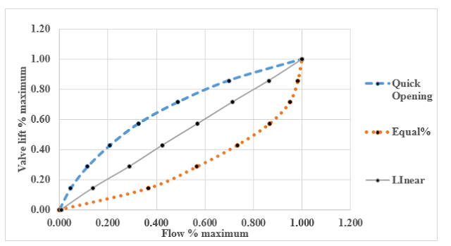 |
Inherent characteristics curves for equal%, linear
and quick opening control valve
|
The above figure show the inherent
characteristics of equal%, linear and quick opening valve. Valve lift in
percentage is represent on y-axis and flow in percentage is represent on the
x-axis.
An equal percentage valve overcompensates
for line loss and produces an effective characteristic that is not linear, but
is bowed in the opposite direction to that of the effective characteristic of
the linear valve. One can show that as the line loss increases, the linear
valve will depart more from the ideal linear relation and the equal percentage
valve will move more closely toward the linear relation. Pressure drop of water
in equal%, quick opening and linear valve are in the range of 101.2 -147.6,
33.6-147.6 and 83.6- 147.6 mm respectively.
7. CONCLUSIONS
It is often stated
in the control literature that the benefit derived from an equal percentage
valve arises from its inherent nonlinear characteristic that compensates for
the line loss to give an effective valve characteristic that is nearly linear. An
equal percentage valve overcompensates for line loss and produces an effective
characteristic that is not linear, but is bowed in the opposite direction to
that of the effective characteristic of the linear valve. One can show that as
the line loss increases, the linear valve will depart more from the ideal
linear relation and the equal percentage valve will move more closely toward
the linear relation.
Pressure
drop of water in equal%, quick opening and linear valve are in the range of
101.2 -147.6, 33.6-147.6 and 83.6- 147.6 mm respectively. Gradually close the
control valve in steps of 4mm of stem travel. The pressure drop across the
valve increases.
8.
References
1. Coughanowr
D., LeBlanc S., ‘Process Systems Analysis and Control’, Mc-Graw Hill Science Engineering
Math, 2nd Edition, 2008, P-300-303.


Sunday, December 16, 2018
CRUDE OIL | Classification of Crude Oil

CRUDE OIL- Classification of Crude Oil
"Crude oil" is usually black or dark brown (although it may be yellowish, reddish, or even greenish). Paraffin base, Naphthene base, asphalt base or mixed base are the "classification of Crude oil". In the reservoir it is usually found in association with natural gas, which being lighter forms a "gas cap" over the petroleum, and saline water which, being heavier than most forms of Crude oil, generally sinks beneath it. "Crude oil" may also be found in a semi-solid form mixed with sand and water. Distillation is used to separate the "Crude oil" into fractions according to boiling point. The crude unit is the first processing unit in the refinery to separate the "Crude oils".
COMPOSITION OF CRUDE OIL
Crude oils are composed of critical homologous series of hydrocarbon. The hydrocarbons present in the crude petroleum are classified into general types-1.1 Paraffin’s
When carbon atom is connected to single bond and other bond are saturated with hydrogen atom.1.2 Olefins
Olefins do not naturally occur in crude oil but are formed during the processing.1.3 Naphthenes
Naphthenes is also known as Cycloparaffins. Cycloparaffin hydrocarbon in which all of the available bonds of the carbon atoms are saturated with hydrogen are called naphthenes.1.4 Aromatics
The aromatics series of hydrocarbon contain a benzene ring which is unsaturated but very stable and frequently behaves as a saturated compound.CLASSIFICATION OF CRUDE OIL
"Crude oils" are classified as paraffin base, Naphthene base, asphalt base or mixed base. The U.S Bureau of mines has developed a system which classifies the crude according to two key fraction obtained in distillation: No 1 from 482 to 527 oF (250 to 275 oC) at atmospheric pressure and No 2 from 527 to 572 oF (275 to 300 oC) at 40 mmHg pressure.
The gravity of these two fractions is used to classify crude oils into types a shown below:
| |||||||||||||||||||||||||||||||||||
The more useful properties are-
3.1 API Gravity
The density of petroleum oils is expressed in the United States in terms of API gravity rather than specific gravity. API is inversely proportional to the specific gravity.
The units of API gravity are oAPI and the relation between API and specific gravity is shown in equation.

In above equation, specific gravity and API gravity refer to the weight per unit volume at 60 oF as compared to water at 60 oF.
3.2 Sulfur Content, wt%
The sulfur content is expressed as percent sulfur by weight and varies from less than 0.1% to greater than 5%. Sulfur content is one of the properties that effect the crude oil prices.
Crude with greater than 0.5% sulfur is more expensive and refers to sour crude oil whereas crude with less than 0.5% sulfur refers to sweet crude.
3.3 Pour point oF or oC
The pour point of the crude oil is a rough indicator of the relative paraffinicity and aromaticity of the crude. The lower the pour point, the lower the paraffin content and the greater the content of aromatics.
3.4 Carbon Residue, wt%
The carbon residue is roughly related to the asphalt content of the crude. And to the quantity of the lubricating oil fraction. Lower the carbon residue, the more valuable the crude.
3.5 Salt content, lb/1000bbl
Crude oil passes through the desalter before going in the Atmospheric distillation if the salt content in the crude is greater than 10lb/ 1000bbl.
Corrosion problem may be encountered, if the salt is not removed. The unit in which salt content measure is PTB.
3.6 Characterization Factors
The Watson characterization factor ranges from less than 10 for highly aromatic materials and 15 for highly paraffinic compounds. Kw vary from 10.5 for a highly naphthenic crude to 12.9 for a paraffinic base crude.
Formula used to calculate the Watson characteristic is given below-

The correlation index is useful in evaluating individual fraction from crude oil. The CI scale is based upon straight-chain paraffins having a CI value of 0 and benzene having a CI value of 100.
Lower the value of CI, the greater the concentration of paraffin hydrocarbon in the fraction, and the higher the CI value, the greater the concentration of naphthenes and aromatics.

3.7 RVP
Reid vapor pressure is approximately the vapor pressure of gasoline at 100 oF3.8 Octane number
Octane number is defined as percentage volume of Iso-octane (2,2,4-trimethyl pentane) in a mixture of iso-octane and n-heptane that gives the same knocking charactristic as the fuel under consideration.3.9 RON
It is research method which represents the performance during city driving when acceleration is relatively frequent3.10 MON
It is Motor method which is the guide to engine performance on the highway or under heavy load condition3.11 Sensitivity
The difference between the research and motor octane number. Low sensitivity is better.
3.12 PON
Posted octane number is arithmetic average of the research and motor octane number.
3.13 Wax Content
The waxes present in most crude oils include n-alkanes, iso-alkanes, alkyl cyclic compounds and alkyl aromatics. In most crude n-alkanes are the predominant species.
There is no standard definition for wax content but it is generally accepted that n-alkanes from C18 to C40 represent waxy material.
Waxy crude oils are highly non-Newtonian materials known to cause handling and pipelining difficulties and whose flow properties are time and history dependent. https://chemengineering1.blogspot.com/2018/10/blog-post.html
3.14 Aniline point
The minimum temperature at which equal volumes of anhydrous aniline and oil mix together. High aniline point indicates that the fuel is highly paraffinic and hence has a high diesel index and very good ignition quality.
3.15 Asphaltenes content
Asphaltenes are composed mainly of polyaromatic carbon ring units with oxygen, nitrogen, and sulfur heteroatoms, combined with trace amounts of heavy metals, particularly chelated vanadium and nickel, and aliphatic side chains of various lengths.
Asphaltenes are defined operationally as the n-heptane (C7H16)-insoluble, toluene soluble component of a carbonaceous material such as crude oil, bitumen, or coal.
3.16 Kinematic Viscosity
Viscosity is a measure of a fluid’s resistance to flow. The term “kinematic” means that the measurement is made while fluid is flowing under the force of gravity. The kinematic viscosity of a fluid is measured in centiStokes.
PROCESS INVOLVED
Crude is heated in the furnace and charged to distillation column where it is separated into butane's and light wet gas is come out from the top and side stream product is come out from the distillation column at different temperature cut.
First cut is naphtha and this naphtha is light also known as light straight run naphtha (LSR). Second cut is heavy straight run naphtha (HSR). Next cut is 380-520 oF which is kerosene. Similarly 520-650 oF , 650-800oF , 800-1000 oF and 1000+ oF cuts are for Light gas oil (LGO), Heavy gas oil (HGO), Vacuum gas oil (VGO) and Vacuum reduced crude (VRC) respectively.

Evaluation of API at different temperature cut
|
At 482 to 527 oF (250 to 275 oC) at atmospheric pressure the API is 34.2 oAPI and at 527 to 572 oF (275 to 300 oC) at 40 mmHg pressure, the API is 30 oAPI therefore from Table 1 Gravity of two fraction to classify crude oil” it’s seem that crude oil is Intermediate, paraffin.
Above Figure shown the TBP and mid-point curve. LSR (C5-190 oF) cut have higher yield than Vacuum residue crude (VRC -1050+ oF). The API gravity increases with
the yield. API is inversely proportional to the specific gravity. Higher the API, more will be lighter components. Lighter cuts have higher yields.
APPENDIX -Tests Methods and Apparatus
Table Properties, ASTM methods and apparatus information
PROPERTY
|
ASTM METHOD
|
APPARATUS
|
Density
|
D4052, D70
|
Digital density meter KYOTO-KEM, Pycnometer
|
Pour Point
|
D5949, D5853
|
Cold flow property analyzer PHASE TECHNOLOGY
|
Water Content
|
D4006, D4928
|
Dean and Stark distillation apparatus, KF Coulometer METROHM
|
Salt Content
|
D3230
|
Salt-in-Crude analyzer KOEHLER
|
Asphaltene Content
|
D3279
|
Automatic asphaltene analyzer COSMO TRADE & SERVICE
|
Wax Content
|
Manual method
| |
Reid Vapor Pressure
|
D323
|
Automated Reid vapor pressure tester WALTER HERZOG GmbH
|
Carbon Residue
|
D4530
|
Micro carbon residue tester
|
Kinematic Viscosity
|
D445, D2170
|
Viscometers CANNON and viscometer holders KOEHLER
|
Flash Point
|
D93
|
Pensky-Martens closed cup flash point tester TANAKA
|
Aniline Point
|
D611
|
Automatic aniline point tester TANAKA
|
Subscribe to:
Posts
(
Atom
)